
Author: Giovanni Pedrelli
Course: Advanced Programming
This repository contains a Jupyter notebook that trains and evaluates a feed-forward supervised Neural Network for a binary classification problem:
- Class 1: signal
- Class 0: background
The workflow reads events from a ROOT file, performs a preliminary analysis of the input variables, prepares a balanced dataset, trains a Keras neural network, and evaluates its performance using several classification metrics and diagnostic plots.
- Introduction
- 1. Project overview
- 2. Workflow
- 3. Dataset
- 4. Input features
- 5. Preliminary analysis
- 6. Data preparation
- 7. Neural-network architecture
- 8. Training configuration
- 9. Main results
- 10. Graphical results
- 11. Repository structure
- 12. Requirements
- 13. How to run the project
- 14. Generated outputs
- 15. Reproducibility and methodological notes
- 16. Possible improvements
- References
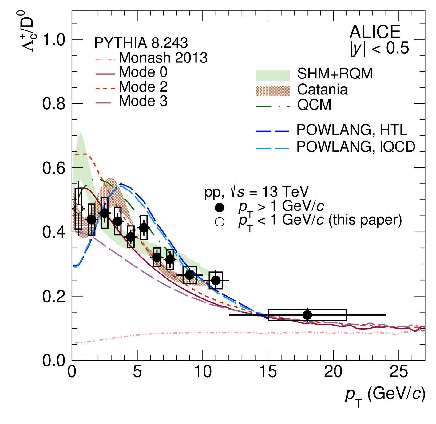
Several models describe the production and behaviour of Quark Gluon Plasma (QGP). Some of them relates it to an enhancement in the production of charmed baryons (baryons with a charm quark) in heavy ion collision experiments.
In the ALICE experiment at CERN, the heavy ion collisions are compared with the proton ones to look for this enhancement.
The measurement of the production cross section of the
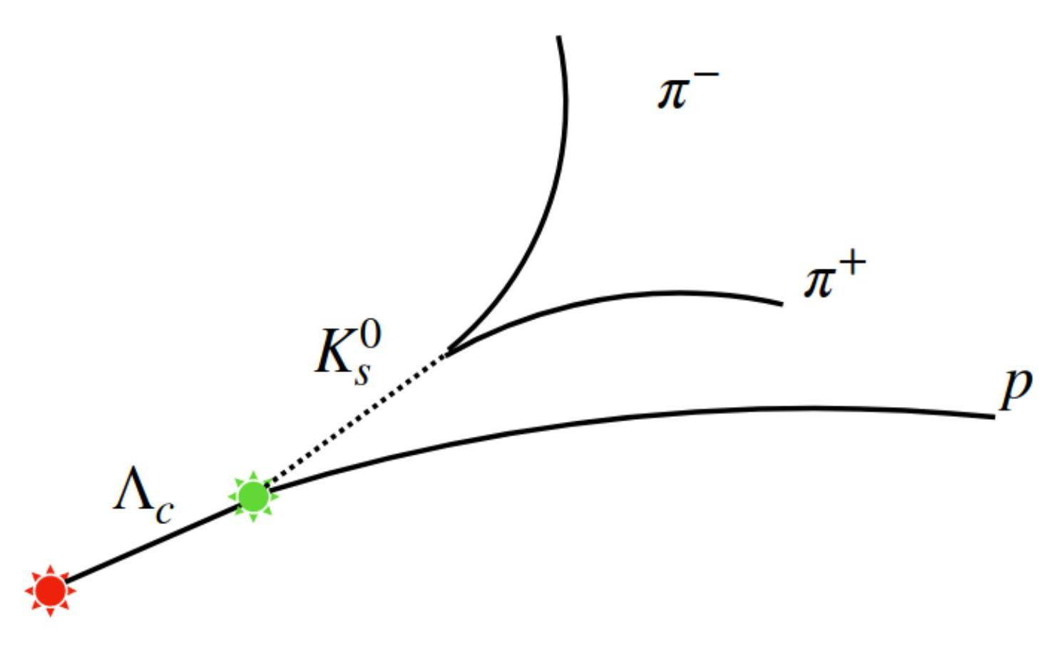
The considered decay channel is
The objective of this project was to develop an independent and customizable machine learning framework for decay analysis and, more generally, for any High Energy Physics (HEP) analysis using the open-source TensorFlow libraries and the Keras APIs. My task has been to build and train the Neural Network.
The dataset used to train the Neural Network contains:
-
simulated signal data generated using simulated proton-proton collision at a center-of-mass energy of
$\sqrt{s} = 13 , \text{TeV}$ ; -
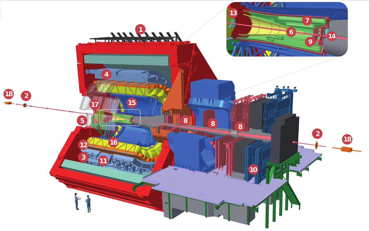
real background data reconstructed using the following ALICE detectors:
- ITS (6 and 7): primary vertex reconstruction and low
$p_T$ tracking; - TPC (15): charged-particle tracking and identification (PID);
- TOF (12): charged-particle identification (PID) through time-of-flight measurements.
- ITS (6 and 7): primary vertex reconstruction and low
The aim of the project is to distinguish signal events from background events when the two classes overlap and cannot be separated effectively using a simple cut on a single variable.
The neural network combines seven input variables and returns, for each event, a value between 0 and 1. This value is interpreted as the model's estimated probability that the event belongs to the signal or the background class.
Using the default classification threshold:
predicted probability >  0.5 → signal
predicted probability <= 0.5 → background
The notebook performs the following steps:
- Imports the required Python modules.
- Creates the dataset directory.
- Downloads the ROOT dataset from Google Drive only when it is missing or incomplete.
- Reads the
TreeSandTreeBtrees using Uproot. - Compares signal and background input-variable distributions.
- Computes separate signal and background correlation matrices.
- Selects and normalizes the input features labelling them as signal or background.
- Balances the dataset by limiting the background sample.
- Splits the data into training and test sets.
- Defines and compiles the neural network.
- Trains the model and records the training history.
- Generates predictions on the test set.
- Computes the ROC curve, confusion matrix, and classification metrics.
- Estimates a simple weight-based feature importance.
- Saves the numerical and graphical results.
The dataset is stored in SB_simul.root.
The notebook checks whether the file already exists and has a size greater than 2 GiB. If this condition is satisfied, the download is skipped. Otherwise, the file is downloaded from Google Drive using gdown.
The ROOT file contains two trees:
| Tree | Meaning |
|---|---|
TreeS |
Signal events (simulated) |
TreeB |
Background events (reconstructed) |
The complete trees contain 13 branches. The model uses only seven of them as input features.
| Sample | Number of events |
|---|---|
| Signal | 943,645 |
| Background used for training and evaluation | 943,645 |
| Total balanced dataset | 1,887,290 |
| Training pool before validation split | 1,509,832 |
| Test set | 377,458 |
The original background tree is considerably larger, so it is truncated to match the number of signal events and create a balanced dataset.
The seven variables used by the neural network are:
| Feature | Physical meaning |
|---|---|
massK0S |
mass of the |
tImpParBach |
impact parameter of the bachelor (the proton) |
tImpParV0 |
impact parameter of the |
CtK0S |
|
cosPAK0S |
|
nSigmapr |
probability for the bachelor to be a proton |
dcaV0 |
minimun distance between the pions produced by the |
- the potentially produced proton is called bachelor
- the potentially produced
$K^0_S$ is called$V^0$
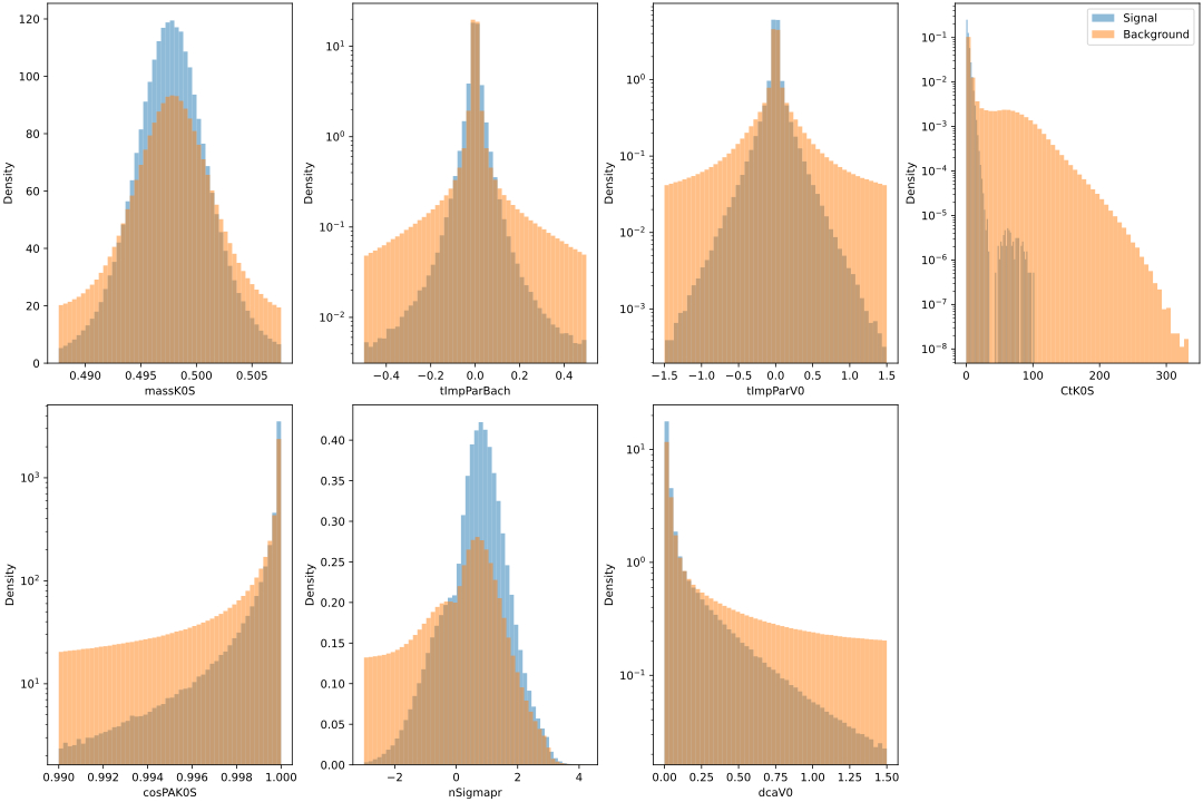
The preliminary analysis compares the signal and background distributions of each variable and examines correlations among the input variables.
The normalized histograms compare the shapes of the signal and background distributions. Variables with visibly different distributions may provide useful discriminating information to the model.
We can also appreciate the necessity of using different techniques from a classic cut, like a neural network, to make the analysis, because the signal and backgound data heavily overlap for each variable.
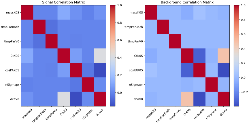
The correlation matrices are calculated separately for signal and background. Differences between the two matrices may provide additional information useful for classification.
The purpose of these plots is to understand whether some input variables carry similar information due to hidden correlations between them. Strongly correlated variables may be partially redundant, while weakly correlated variables may provide more independent information to the neural network.
The target array is defined as:
1 → signal
0 → background
A "target" column is added to the data to distinguish signal (1) from background (0), labelling the data for SUPERVISED LEARNING
np.concatenate([
    np.ones(len(X_signal_normalized)),
    np.zeros(len(X_background_normalized[:bkg_max]))
])Each variable is divided by its maximum value. Signal and background are normalized separately before being concatenated.
The balanced dataset is divided using:
train_test_split(
    X,
    y,
    test_size=0.2,
    random_state=42,
    shuffle=True
)
Therefore:
- 80% of the complete dataset is assigned to the training pool.
- 20% is assigned to the independent test set.
- During
model.fit(), 20% of the training pool is used as validation data.
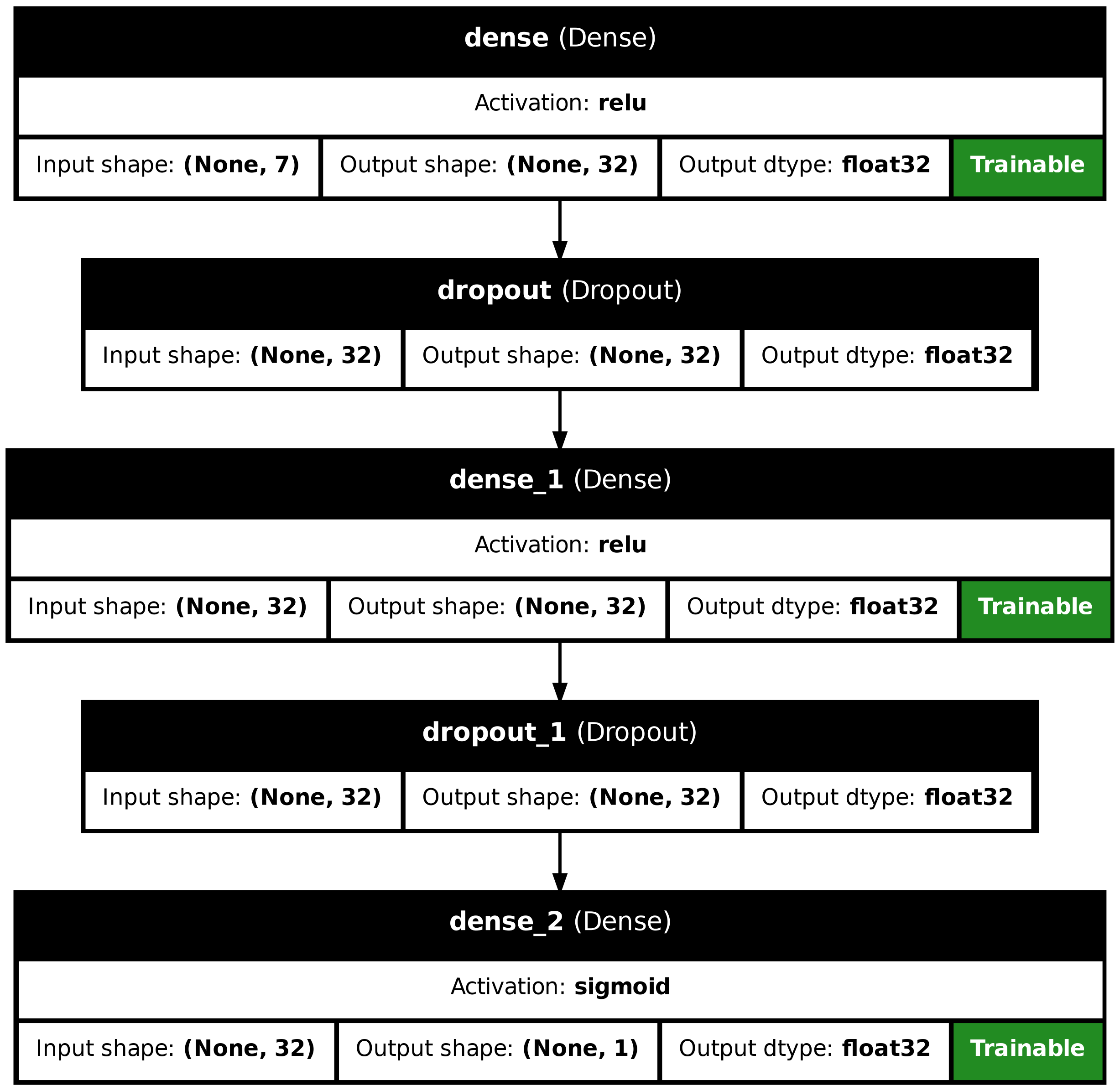
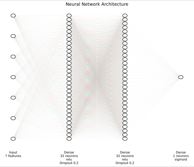
The model is implemented using the Keras Sequential API.
Input: 7 features
        ↓
Dense: 32 neurons, ReLU
        ↓
Dropout: 0.2
        ↓
Dense: 32 neurons, ReLU
        ↓
Dropout: 0.2
        ↓
Output: 1 neuron, sigmoid
| Layer | Output size | Activation | Parameters |
|---|---|---|---|
| Input | 7 | — | 0 |
| Dense | 32 | ReLU | 256 |
| Dropout | 32 | — | 0 |
| Dense | 32 | ReLU | 1,056 |
| Dropout | 32 | — | 0 |
| Dense output | 1 | Sigmoid | 33 |
| Total | — | — | 1,345 |
- The two hidden dense layers learn nonlinear combinations of the input variables.
- The dropout layers randomly set 20% of their inputs to zero during training to reduce overfitting.
- The final sigmoid neuron produces a value between 0 and 1.
| Hyperparameter | Value |
|---|---|
| Hidden layers | 2 |
| Neurons per hidden layer | 32 |
| Hidden activation | ReLU |
| Dropout rate | 0.2 |
| Output activation | Sigmoid |
| Optimizer | Adam |
| Learning rate | 0.001 |
| Loss function | Binary cross-entropy |
| Batch size | 32 |
| Epochs | 10 |
| Validation split | 0.2 |
| Classification threshold | 0.5 |
The monitored metrics are:
- accuracy;
- precision;
- recall;
- loss;
- validation accuracy;
- validation precision;
- validation recall;
- validation loss.
The F1-score is calculated from precision and recall after training.
For a typical run:
Training time: 269.69 seconds
Wall time: approximately 4 minutes and 29 seconds
Execution time can vary depending on the processor, available memory, TensorFlow version, and GPU availability.
The following values refer to a typical notebook output.
| Metric | Value | Percentage |
|---|---|---|
| Accuracy | 0.812983 | 81.30% |
| Precision for signal | 0.805233 | 80.52% |
| Recall / signal efficiency | 0.826018 | 82.60% |
| F1-score | 0.815493 | 81.55% |
| ROC AUC | 0.904289 | 90.43% |
| Background rejection at threshold 0.5 | 0.799930 | 79.99% |
| False-positive rate at threshold 0.5 | 0.200070 | 20.01% |
- The accuracy indicates that approximately 81.3% of all test events are classified correctly.
- The precision indicates that approximately 80.5% of the events classified as signal are actually signal.
- The recall indicates that approximately 82.6% of the true signal events are recovered.
- The F1-score summarizes the balance between precision and recall.
- The ROC AUC indicates good overall separation between signal and background over all possible classification thresholds.
- At the threshold of 0.5, approximately 80.0% of the background events are correctly rejected.
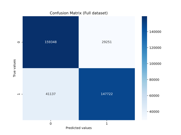
Rows correspond to true classes (wrote in the labels) and columns correspond to predicted classes (classified by the neural network).
| Predicted background | Predicted signal | |
|---|---|---|
| True background | TN = 150.866 | FP = 37.733 |
| True signal | FN = 32.858 | TP = 156.001 |
| Class | Precision | Recall | F1-score | Support |
|---|---|---|---|---|
Background (0) |
0.82 | 0.80 | 0.81 | 188,599 |
Signal (1) |
0.81 | 0.83 | 0.82 | 188,859 |
| Overall accuracy | — | — | 0.81 | 377,458 |
The support column shows the number of total events belonging to that regardless of the classification (correct of incorrect).
The exact values may change slightly between runs because the TensorFlow random seed is not explicitly fixed in the notebook.
10.1 ROC (Receiver Operating Characteristic) curve and AUC: signal efficiency and background rejection
The curve plots signal efficiency, equivalent to the true-positive rate, against background rejection, defined as 1 - FPR, for different classification thresholds.
ROC AUC means Area Under the ROC Curve.
It is a single number that summarizes the overall ability of the model to separate the two classes, signal and background.
roc_auc = 1.0 → perfect separation
roc_auc = 0.5 → random guessing
roc_auc < 0.5 → worse than random guessing
ROC AUC in our case is 0.9043 so it's quite good.
Higher ROC AUC means that the model is better at assigning higher probabilities to signal events than to background events.

The notebook estimates feature importance using the mean absolute first-layer weight associated with each input feature.
For a typical run, the approximate ranking is:
| Rank | Feature | Mean absolute first-layer weight |
|---|---|---|
| 1 | CtK0S |
5.195956 |
| 2 | tImpParV0 |
0.802650 |
| 3 | dcaV0 |
0.729950 |
| 4 | tImpParBach |
0.282166 |
| 5 | nSigmapr |
0.225817 |
| 6 | massK0S |
0.214017 |
| 7 | cosPAK0S |
0.177059 |
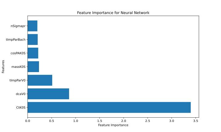
This feature-importance method is a heuristic based only on the first-layer weights. It should not be interpreted as a causal or definitive measure of physical importance.
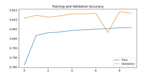

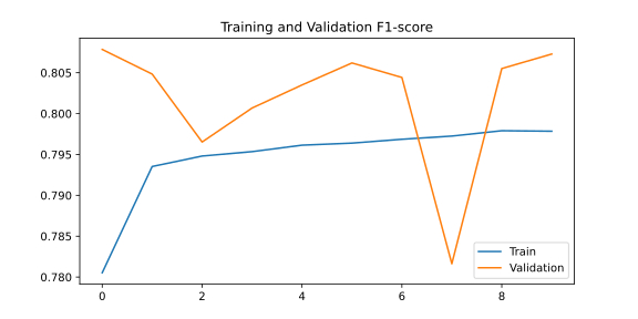
The repository structure is the following (inside the folders there will be the output files):
.
├── README.md
├── NN.ipynb
├── nn.dockerfile
├── dataset/
│   └── SB_simul.root
├── preliminary_analysis/
├── model_drawings/
└── evaluation_results/
The ROOT dataset is large and is not committed to GitHub, the same holds for compiled, generated, results files. So everything is setup in the .gitignore file.
The notebook uses the following main packages:
numpy
uproot
pandas
seaborn
matplotlib
tensorflow
scikit-learn
gdown
awkward
The Keras layer diagram additionally requires:
pydot
graphviz
Everything is already downloaded in the nn.dockerfile.
cd ~/ && git clone https://github.com/giopedro92/advanced-programming-project.git && cd ~/advanced-programming-projectsudo docker build -f nn.dockerfile -t nn .- To execute the image to create the container and access it via a browser
sudo docker run --rm -p 8888:8888 -v ~/advanced-programming-project/:/home/jovyan/ nn- To execute the image to create the container accessing it via VSCode
sudo docker run -it --rm -p 8888:8888 -v ~/advanced-programming-project/:/home/jovyan/ nn jupyter notebook --ip 0.0.0.0Run the notebook from top to bottom. The needed files, the generated directories and the result files are downloaded or created automatically.
This file contains:
- accuracy;
- F1-score;
- precision;
- ROC AUC;
- all FPR and TPR pairs used for the ROC analysis.
The train/test split is reproducible because random_state=42 is used. However, TensorFlow's random seed is not explicitly fixed, so network initialization, dropout masks, and final numerical results may vary slightly.
The current feature importance is based on the average absolute weights of the first dense layer. This is useful as a quick diagnostic, but it does not fully capture nonlinear interactions among features.
More robust alternatives include:
- permutation importance;
- SHAP values;
- feature ablation studies.
The reported confusion matrix and threshold-dependent metrics use a fixed threshold of 0.5. A different threshold may be preferable depending on the required trade-off between signal efficiency and background rejection.
Potential extensions include:
- selecting the classification threshold according to the physics objective;
- using early stopping;
- saving the trained model;
- comparing the neural network with simpler baseline classifiers;
- tuning the number of neurons, dropout rate, learning rate, and batch size;
- applying the trained network on real data to make predictions (!).